Optical Loss Budgets

The optical loss budget is an important aspect in designing networks with the Cisco ONS 15540. The optical loss budget is the ultimate limiting factor in distances between nodes in a topology. This chapter contains the following major sections:

Note The optical specifications described in this chapter are only for the individual components and should not be used to characterize the entire network performance.

Note The information in this chapter applies only to nonamplified network design.

About dB and dBm

Signal power loss or gain is never a fixed amount of power, but a portion of power, such as one-half or one-quarter. To calculate lost power along a signal path using fractional values you cannot add 1/2 and 1/4 to arrive at a total loss. Instead, you must multiply 1/2 by 1/4. This makes calculations for large networks time-consuming and difficult.

For this reason, the amount of signal loss or gain within a system, or the amount of loss or gain caused by some component in a system, is expressed using the decibel (dB). Decibels are logarithmic and can easily be used to calculate total loss or gain just by doing addition. Decibels also scale logarithmically. For example, a signal gain of 3 dB means that the signal doubles in power; a signal loss of 3 dB means that the signal halves in power.

Keep in mind that the decibel expresses a ratio of signal powers. This requires a reference point when expressing loss or gain in dB. For example, the statement "there is a 5 dB drop in power over the connection" is meaningful, but the statement "the signal is 5 dB at the connection" is not meaningful. When you use dB you are not expressing a measure of signal strength, but a measure of signal power loss or gain.

It is important not to confuse decibel and decibel milliwatt (dBm). The latter is a measure of signal power in relation to 1 mW. Thus a signal power of 0 dBm is 1 mW, a signal power of 3 dBm is 2 mW, 6 dBm is 4 mW, and so on. Conversely, -3 dBm is 0.5 mW, -6 dBm is 0.25 mW, and so on. Thus the more negative the dBm value, the closer the power level approaches zero.

Overall Optical Loss Budget

An optical signal degrades as it propagates through a network. Components such as optical mux/demux modules, fiber, fiber connectors, splitters, and switches introduce attenuation. Ultimately, the maximum allowable distance between the transmitting laser and the receiver is based upon the optical link budget that remains after subtracting the power losses experienced by the channels with the worst path as they traverse the components at each node.

Table 4-1 lists the laser transmitter power and receiver sensitivity range for the data channels and the OSC (Optical Supervisory Channel).

Table 4-1 Trunk Side Transmitter Power and Receiver Ranges
Channel	Transmit Power (dBm)		Receiver Sensitivity (dBm)
Channel	Minimum	Maximum	Minimum	Overload
SM transponder module and MM transponder module data channel	4	8	-28	-8
Extended range transponder module data channel	5	10	-28	-8
OSC	4	8	-19	-1.5

Note Add the proper system-level penalty to the receive power based on your actual network topology characteristics, such as dispersion.

The goal in calculating optical loss is to ensure that the total loss does not exceed the overall optical link (or span) budget. For the Cisco ONS 15540, this is 38 dB for data channels. For example, the OSC has an optical link budget of 26 dB, which is equal to the OSC receiver sensitivity (-22 dBm) subtracted from the OSC laser launch power (4 dBm) on the mux/demux motherboard. Typically, in point-to-point topologies, the OSC optical power budget is the distance limiting factor, while in ring topologies, the data channel optical power budget is the distance limiting factor.

Calculating Optical Loss Budgets

Using the optical loss characteristics for the Cisco ONS 15540 components, you can calculate the optical loss between the transmitting laser on one node and the receiver on another node. The general rules for calculating the optical loss budget are as follows:

•

The maximum power loss between the nodes cannot exceed the minimum transmitter power of the laser minus the minimum sensitivity of the receiver and network-level penalty.

Note

Determine the proper network-level penalty to the receive power based on your actual network topology characteristics, such as dispersion.

•

The minimum attenuation between the nodes must be greater than the maximum transmitter power of the laser minus the receiver overload value.

The following example shows how to calculate the optical loss budget for 2.5-Gbps data channels from an extended range transponder module using the values in Table 4-1:

•

The power loss between the transmitter laser and receiver must not exceed 33 (5 - (-28)) dB or the signal will not be detected accurately.

•

At least 18 (10 - (-8)) dB of attenuation between neighboring nodes prevents receiver saturation.

To validate a network design, the optical loss must be calculated for each band of channels. This calculation must be done for both directions if protection is implemented, and for the OSC between each pair of nodes. The optical loss is calculated by summing the losses introduced by each component in the signal path.

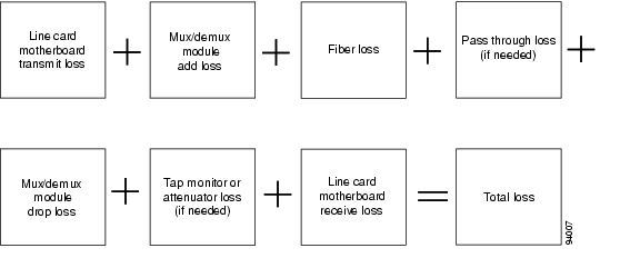
At a minimum, any data channel path calculation must include line card transmit loss, channel add loss, fiber loss, channel drop loss, and line card receive loss (see Figure 4-1). In ring topologies, pass through losses must be considered. Losses due to external devices such as fixed attenuators and monitoring taps must also be included.

Optical Loss for 2.5-Gbps Line Card Motherboards

In the transmit direction, the splitter protected line card motherboard attenuates the ITU signal emitted from its associated transponders significantly more than does the east or west motherboard. In the receive direction, the splitter protected line card motherboard attenuates the signal destined for its associated transponder significantly more than does the east or west motherboard.

Table 4-2 shows the optical loss for the splitter protected, east, and west motherboards in the transmit and receive directions.

Table 4-2 Optical Loss for 2.5-Gbps Line Card Motherboards
Line Card Motherboard Type and Direction	Loss (dB)
Splitter protected motherboard Tx	4.6
Splitter protected motherboard Rx	1.9
East motherboard Tx	1.0
East motherboard Rx	1.0
West motherboard Tx	1.0
West motherboard Rx	1.0

Optical Loss for Optical Mux/Demux Modules

Optical mux/demux modules attenuate the signals as they are multiplexed, demultiplexed, and passed through. The amount of attenuation depends upon the type of optical mux/demux module and the path the optical signal takes through the modules.

Loss for Data Channels

Table 4-3 shows the optical loss for the data channels between the 4-channel or 8-channel add/drop mux/demux modules and the transponders, and between the pass through add and drop connectors on the modules.

Table 4-3 Optical Loss for Data Channels Through the Add/Drop Mux/Demux Modules
Optical Mux/Demux Module Type	Trunk IN to Line Card Motherboard (Data Drop) in dB	Line Card Motherboard to Trunk OUT (Data Add) in dB	Trunk IN to Thru OUT (Pass Through Drop) in dB	Thru IN to Trunk OUT (Pass Through Add) in dB
4-channel with OSC	4.1	4.1	1.5	1.5
8-channel with OSC	4.8	4.8	2.0	2.0
4-channel without OSC	4.1	4.1	1.0	1.0
8-channel without OSC	4.8	4.8	1.5	1.5

Table 4-4 list the optical loss for the 16-channel terminal mux/demux modules. The third row of the table lists the connector loss and total loss when the two 16-channel modules are cascaded to support 32 channels.

Table 4-4 Optical Loss for Data Channels Through the Terminal Mux/Demux Modules
Loss Source	IN to Line Card Motherboard (Data Drop) in dB	Line Card Motherboard to OUT (Data Add) in dB
16-channel with OSC (channels 1-16)	6.5	6.5
16-channel without OSC (channels 17-32)	6.5	6.5
Total loss (32 channels)	6.5	6.5

Note The insertion losses listed in Table 4-3 and Table 4-4 are worst case values. Take this into consideration when calculating the minimum loss budget.

Loss for the OSC

Table 4-5 shows the optical loss for the OSC between the mux/demux motherboard and the optical mux/demux modules.

Table 4-5 Optical Loss for the OSC Through the Optical Mux/Demux Modules
Optical Mux/Demux Module Type	Trunk IN to OSC Transceiver (dB)	OSC Transceiver to Trunk OUT (dB)
4-channel with OSC	2.8	2.8
8-channel with OSC	3.3	3.3
16-channel with OSC	7.1	7.1

Fiber Plant Testing

Verifying fiber characteristics to qualify the fiber in the network requires proper testing. This document describes the test requirements but not the actual procedures. After finishing the test measurements, compare the measurements with the specifications from the manufacturer, and determine whether the fiber supports your system requirements or whether changes to the network are necessary.

This test measurement data can also be used to determine whether your network can support higher bandwidth services such as 10 Gigabit Ethernet, and can help determine network requirements for dispersion compensator modules or amplifiers.

.Fiber optic testing procedures must be performed to measure the following parameters

Link Loss (Attenuation)

Testing for link loss, or attenuation, verifies whether fiber spans meet loss budget requirements.

Attenuation includes intrinsic fiber loss, losses associated with connectors and splices, and bending losses due to cabling and installation. An OTDR (optical time domain reflector/reflectometer) is used when a comprehensive accounting of these losses is required. The OTDR sends a laser pulse through each fiber; both directions of the fiber are tested at 1310 nm and 1550 nm wavelengths.

OTDRs also provide information about fiber uniformity, splice characteristics, and total link distance. For the most accurate loss test measurements, an LTS (loss test set) that consists of a calibrated optical source and detector is used. However, the LTS does not provide information about the various contributions (including contributions related to splice and fiber) to the total link loss calculation.

A combination of OTDR and LTS tests is needed for accurate documentation of the fiber facilities being tested. In cases where the fiber is very old, testing loss as a function of wavelength (also called spectral attenuation) might be necessary. This is particularly important for qualifying the fiber for multiwavelength operation. Portable chromatic dispersion measurement systems often include an optional spectral attenuation measurement.

ORL

ORL is a measure of the total fraction of light reflected by the system. Splices, reflections created at optical connectors, and components can adversely affect the behavior of laser transmitters, and they all must be kept to a minimum of 24 dB or less. You can use either an OTDR or an LTS equipped with an ORL meter for ORL measurements. However, an ORL meter yields more accurate results.

PMD

PMD has essentially the same effect on the system performance as chromatic dispersion, which causes errors due to the "smearing" of the optical signal. However, PMD has a different origin from chromatic dispersion. PMD occurs when different polarization states propagate through the fiber at slightly different velocities.

PMD is defined as the time-averaged DGD (differential group delay) at the optical signal wavelength. The causes are fiber core eccentricity, ellipticity, and stresses introduced during the manufacturing process. PMD is a problem for higher bit rates (10 GE and above) and can become a limiting factor when designing optical links.

The time-variant nature of dispersion makes it more difficult to compensate for PMD effects than for chromatic dispersion. "Older" (deployed) fiber may have significant PMD—many times higher than the 0.5 ps/� km specification seen on most new fiber. Accurate measurements of PMD are very important to guarantee operation at 10 Gbps. Portable PMD measuring instruments have recently become an essential part of a comprehensive suite of tests for new and installed fiber. Because many fibers in a cable are typically measured for PMD, instruments with fast measurement times are highly desirable.

Chromatic Dispersion

Chromatic dispersion testing is performed to verify that measurements meet your dispersion budget.

Chromatic dispersion is the most common form of dispersion found in single-mode fiber. Temporal in nature, chromatic dispersion is related only to the wavelength of the optical signal. For a given fiber type and wavelength, the spectral line width of the transmitter and its bit rate determine the chromatic dispersion tolerance of a system.

Portable chromatic dispersion measurement instruments are essential for testing the chromatic dispersion characteristics of installed fiber.

Table Of Contents